3D isovists

In this tutorial, the idea is to explore the potential of Isovist for urban analysis. Isovist is the surface or volume of space visible from a specific point. This concept has been proposed by Clifford Tandy in 1967 and then redefined by Michael Benedikt. Isovists are very useful to quantify the perception of urban spaces such as opening, closeness, and also useful to define urban envelopes. Isovists help to with non-intuitive solutions for complex problems.

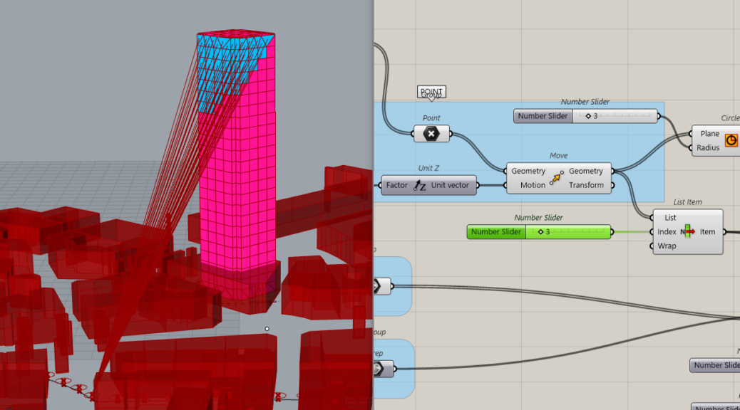
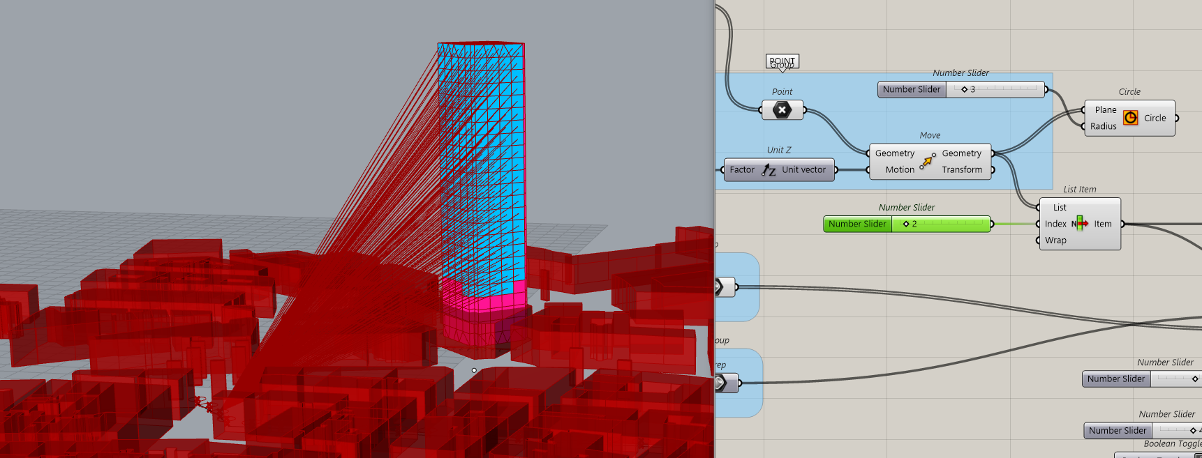
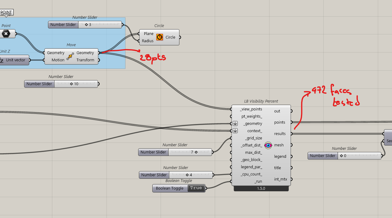
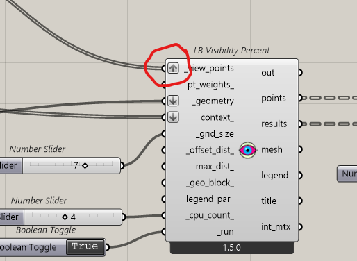
Now we want to do the same in 3D. We will use the Ladybug components. We will use the LB visibility percent.

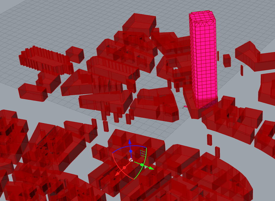
We will investigate how much the tower is seen.

The previous Isovist system will not be used anymore. We just keep the point. Then we connect as shown…context is context and the tower wil be our geometry.

We click on the Boolean Toggle to start the simulation

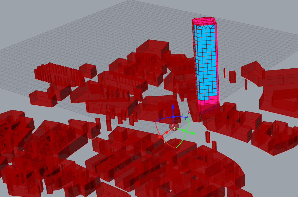
This is how the Tower is seen from this location

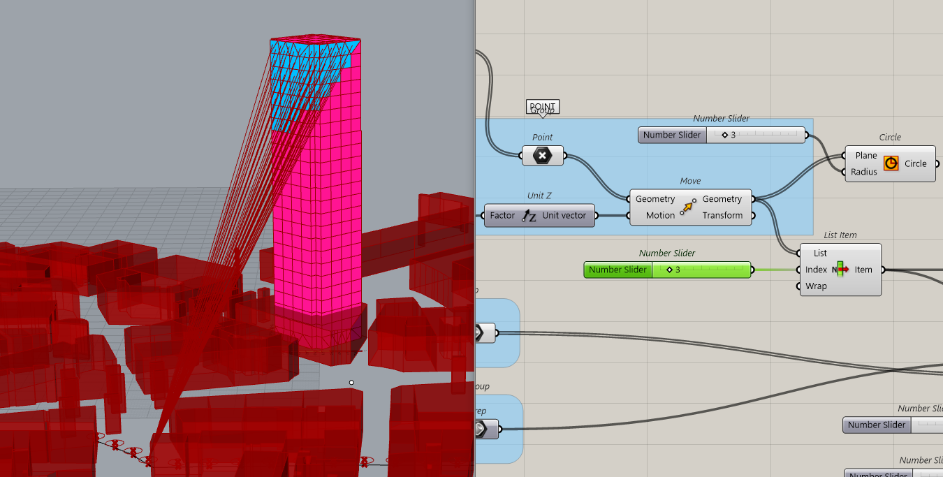
If we go in a narrow street…the tower is no more visible despite the fact that it is super high.

Exploring along a path

Now we could try to see what is happening when we walk in the street, how often we see this huge tower.

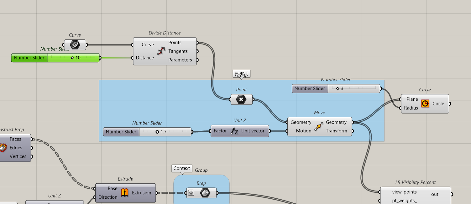
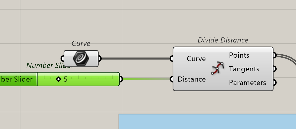
We create a line that we will divide by distance, saying we test every 5 meters, or more or less….

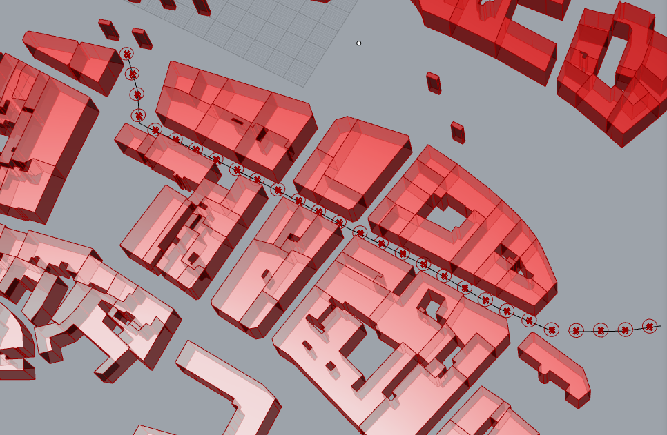
Let’s try

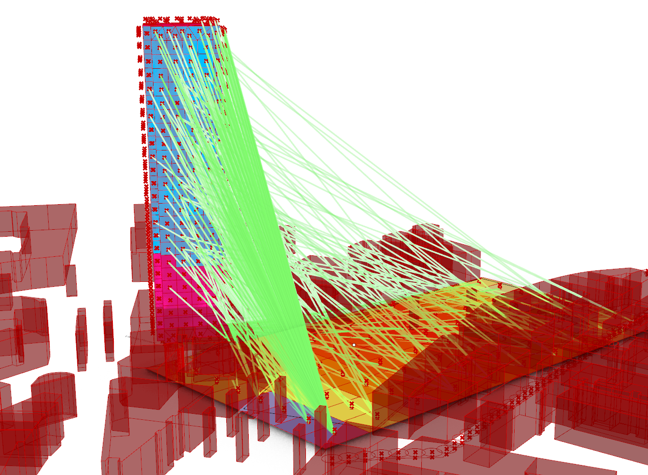
We can try to see for every step how the façade is seen, we can draw the lines of sight.

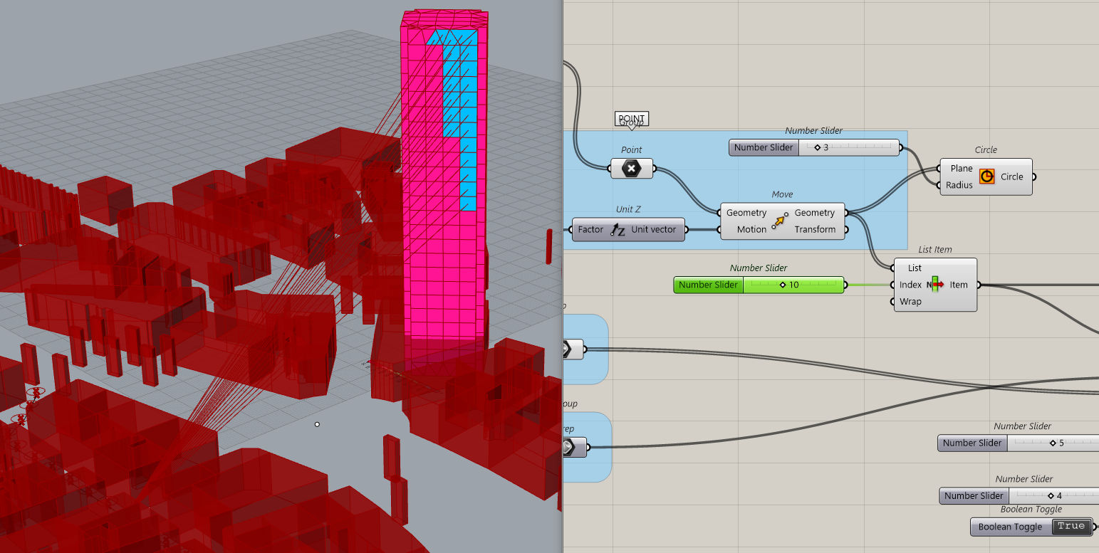
This is the visibility for point n°2

This is n°3

N°10 as 6,7,8,9 don’t see nothing

To prepare that, we just sort the points with 0 visibility from the others…

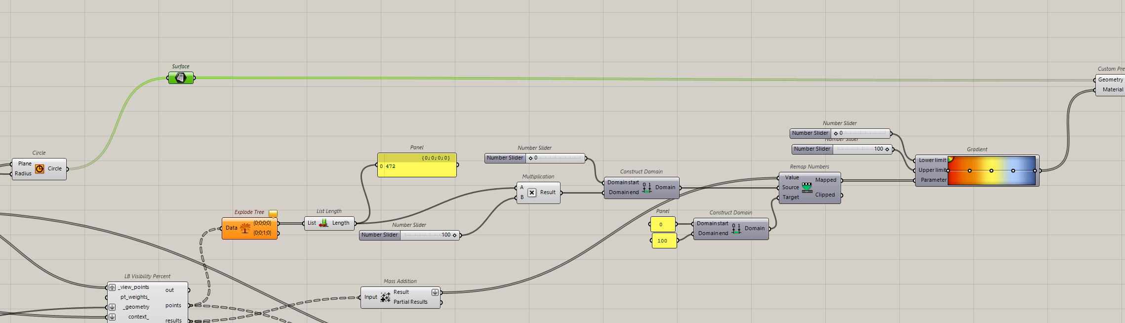
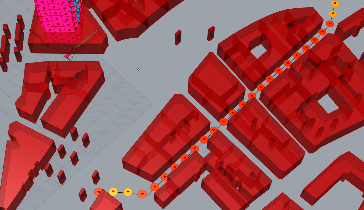
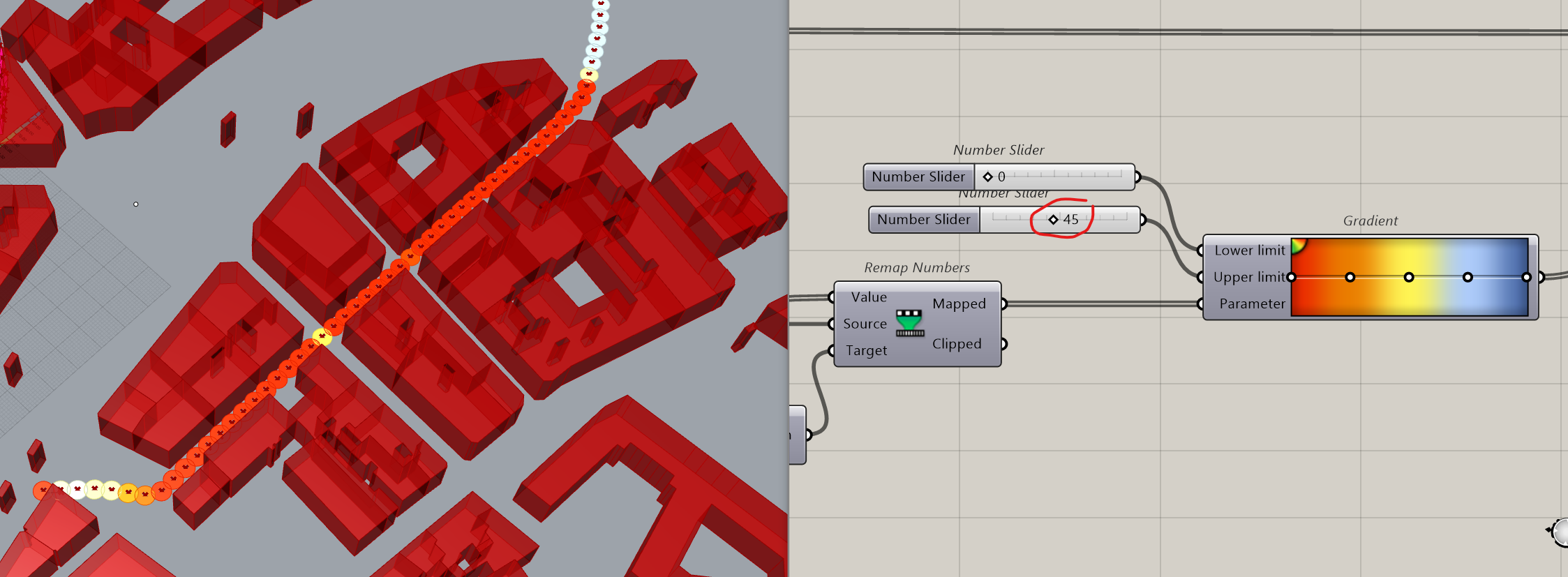
Mapping the visibility

Now, we will try to have a global view of the visibility from the path itself. It means that we want to see with a colour code when we do see the tower and when it’s masked. To do that, we will affect to the circles a specific colour, for instance, red, no visibility, and yellow partial, blue full visibility. Blue will never happened as it is not possible to see all sides of the tower at once.

Ok, the best score would be 100. The chosen grid size gives a certain amount of faces to be investigated.

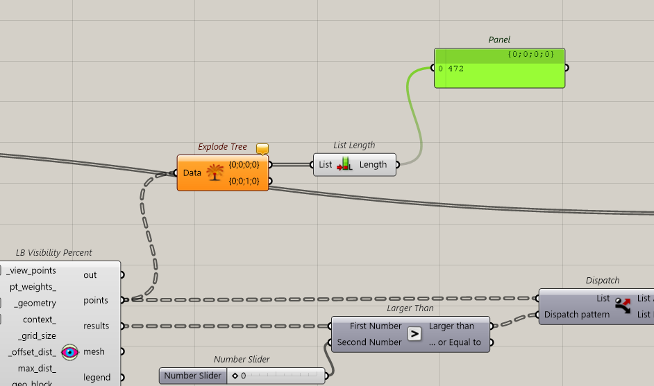
Now we have 28 points on our path and 472 spots to test on the building.

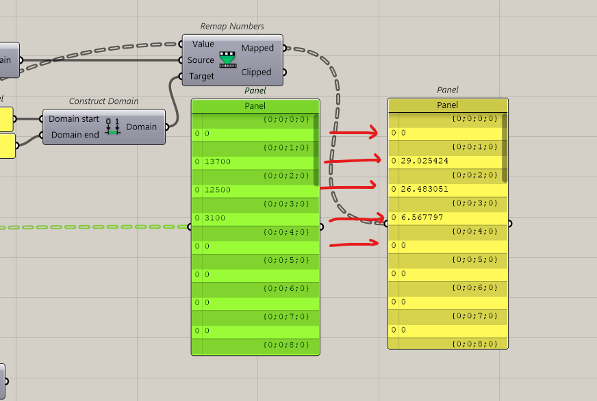
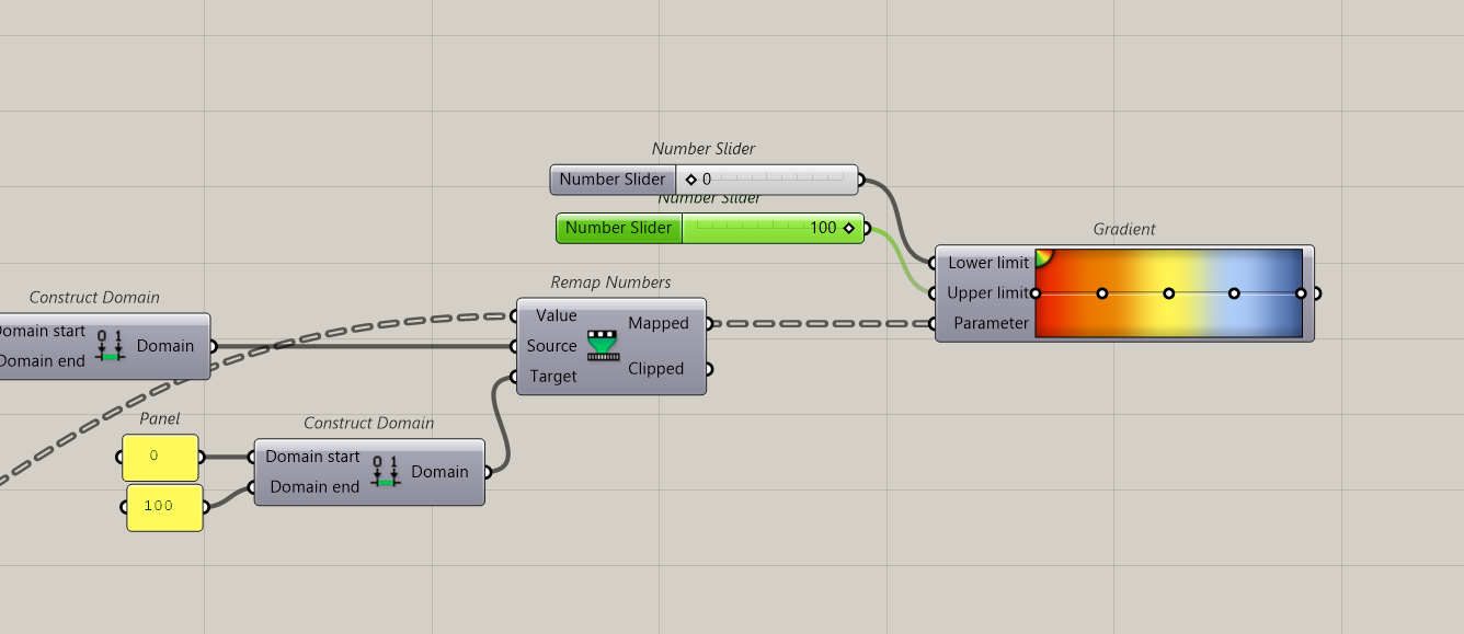
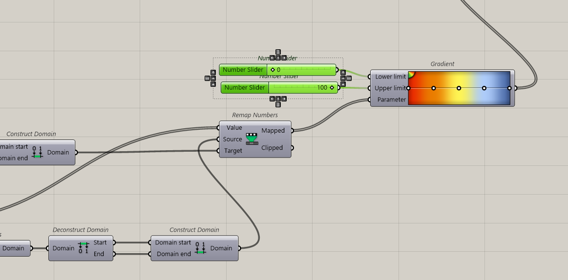
We have to test every point on the path, get the result, and transform it into a colour. For that we need a domain. We associate a gradient of colours to a gradient of values. 1 number = 1 colour.

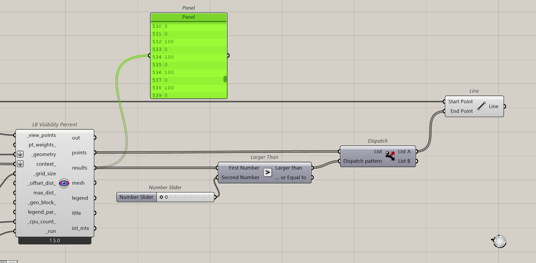
We graph the flux of points, so that every point on the path will be tested and then the next and so on.

We extract the number of points tested on the tower

But as we graphed, we must take the first iteration only, not the whole repeated process…

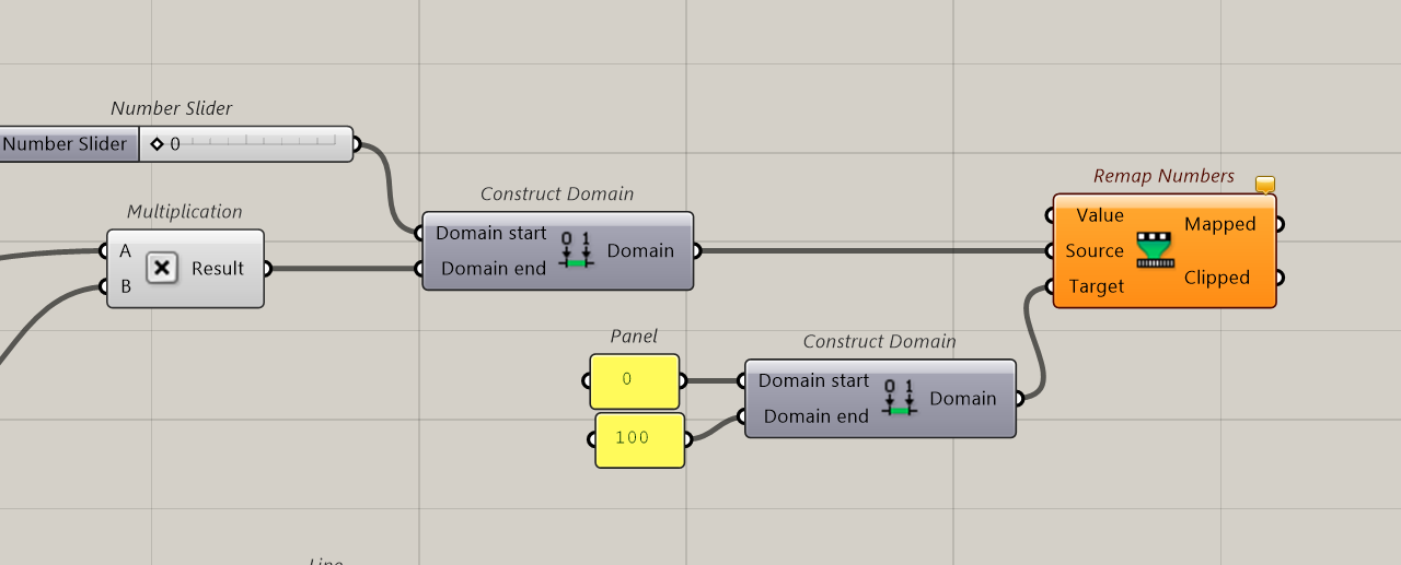
Then we will create a domain. Upper limit, the best score possible, lower, the worst and our results will be in between.

The best theoretical result is number of points on the tower multiply by 100. This is the domain end (best score). The domain starts with 0.

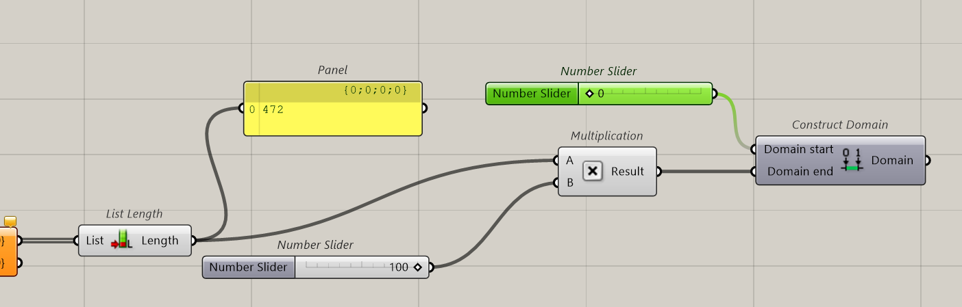
Ok now we’ve got our max and min numbers. To make things simple, we can remap this domain from 0 to 100. Like a percentage.

Now we just have to input the calculated values.

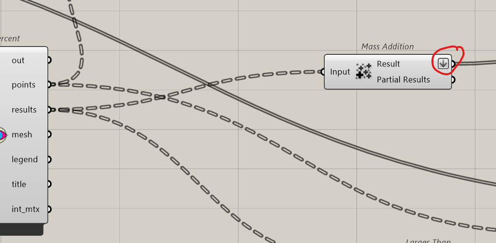
In the results, we have the score for each tested point. So we add everything (Mass addition). And we connect that to value. Attention, Mass Addition result has to be flatten.

Let’s check:

Ok, now we affect a colour for each value according to a gradient.

We set a custom preview, input geometry will be the circles, and colours from gradient. For each point from the path, we check the value and the correspondent colour.

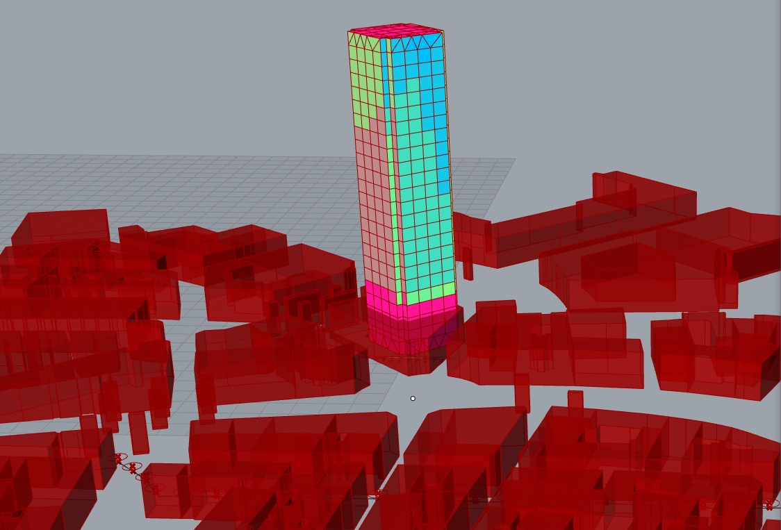
Now we see the result

To have more details, we can test more points on the path, every 5 meters

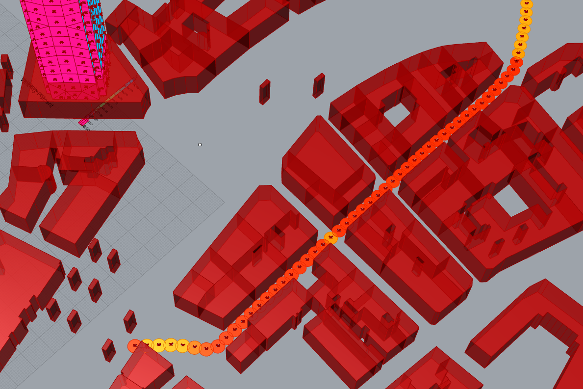
We can also decrease the Upper limit to have more nuances.

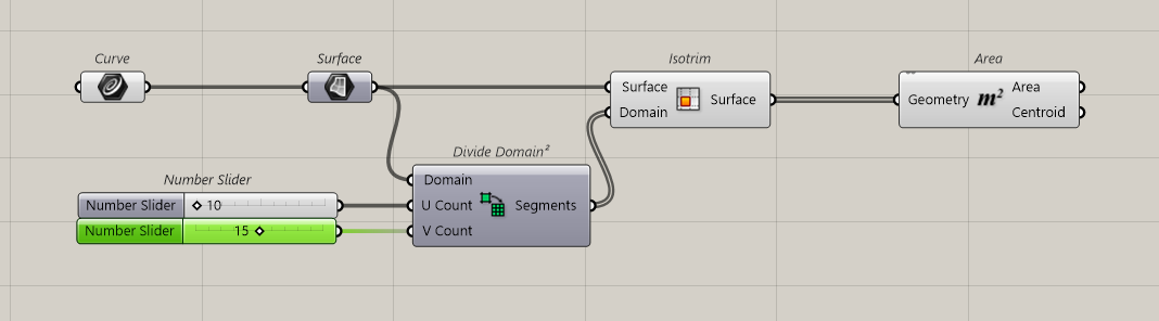
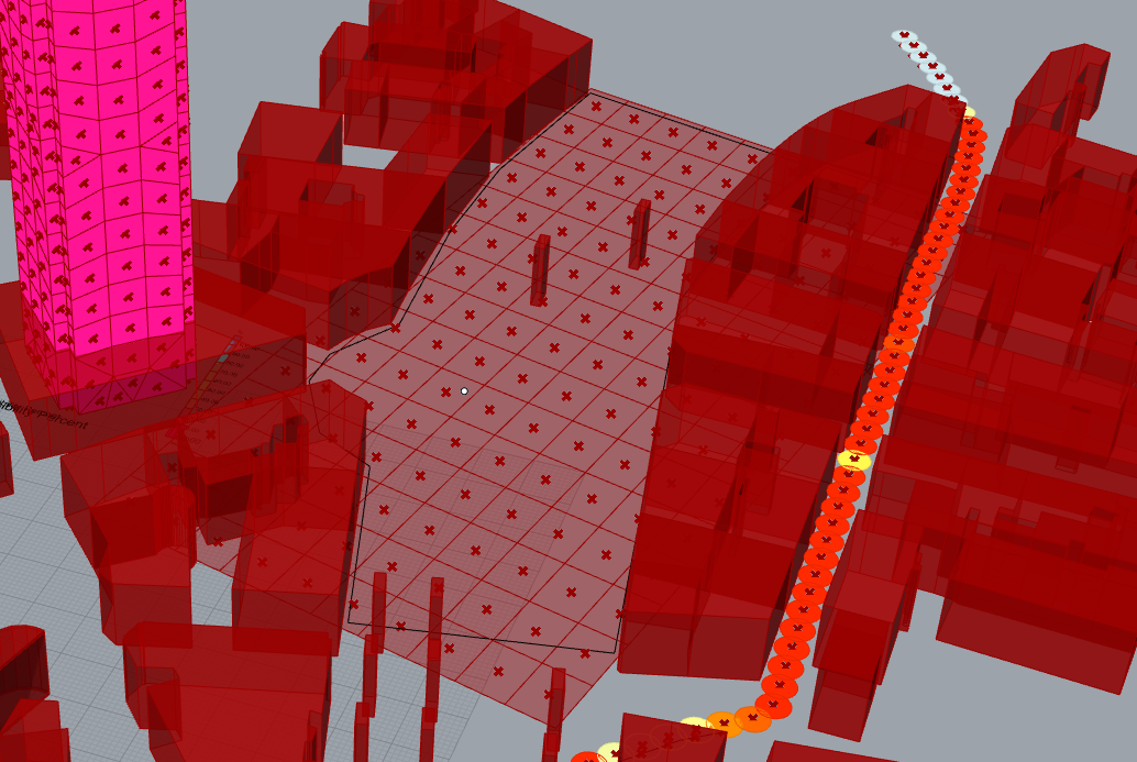
Investigating a Surface

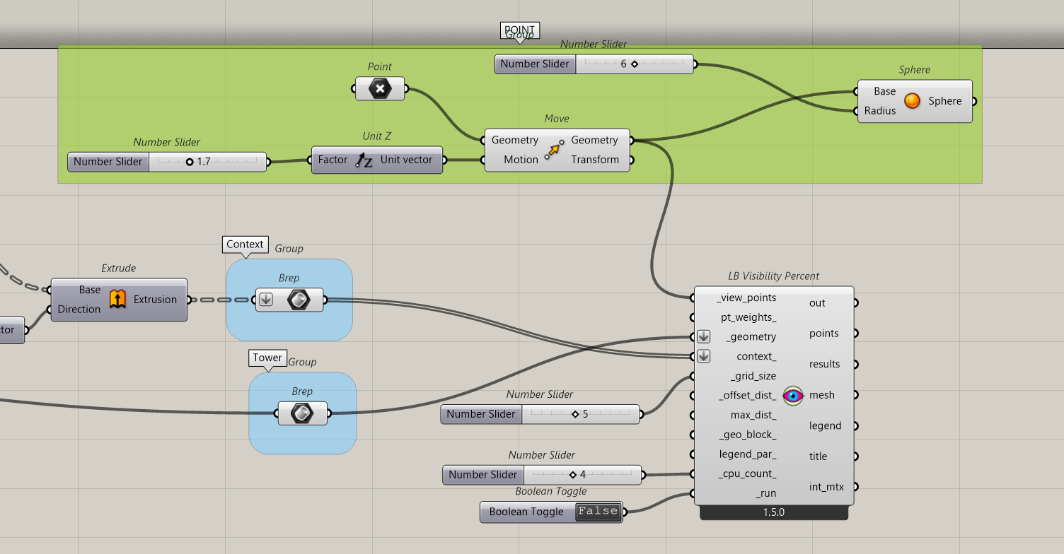
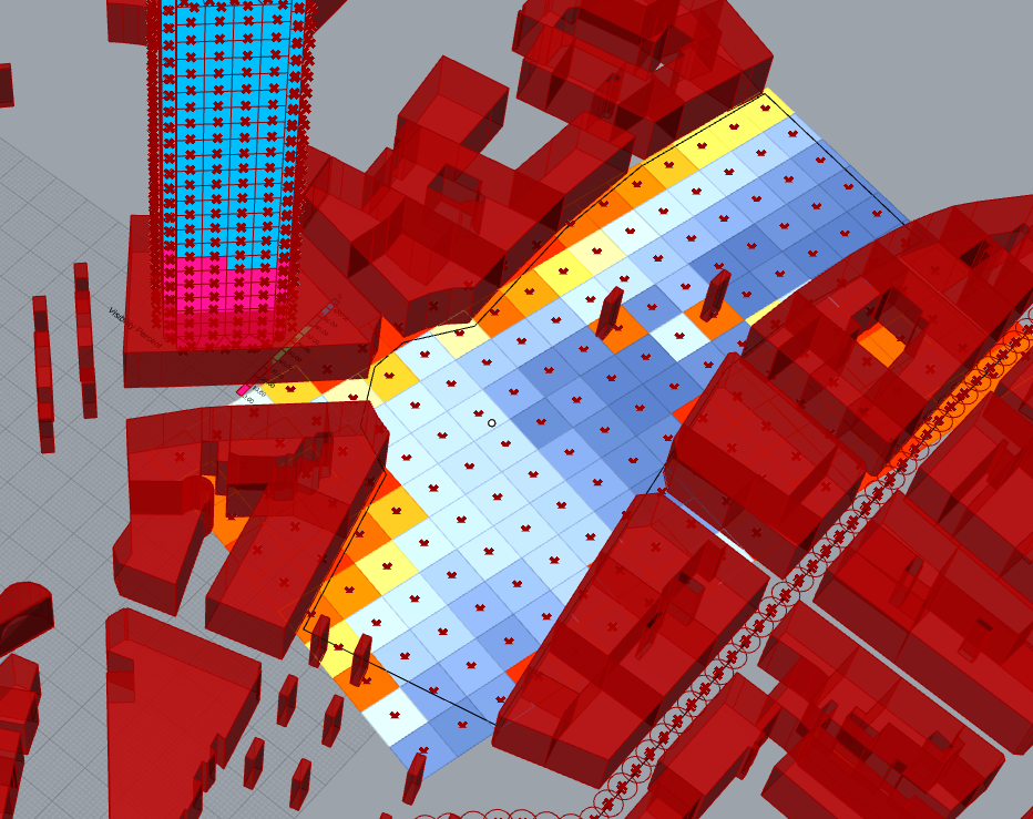
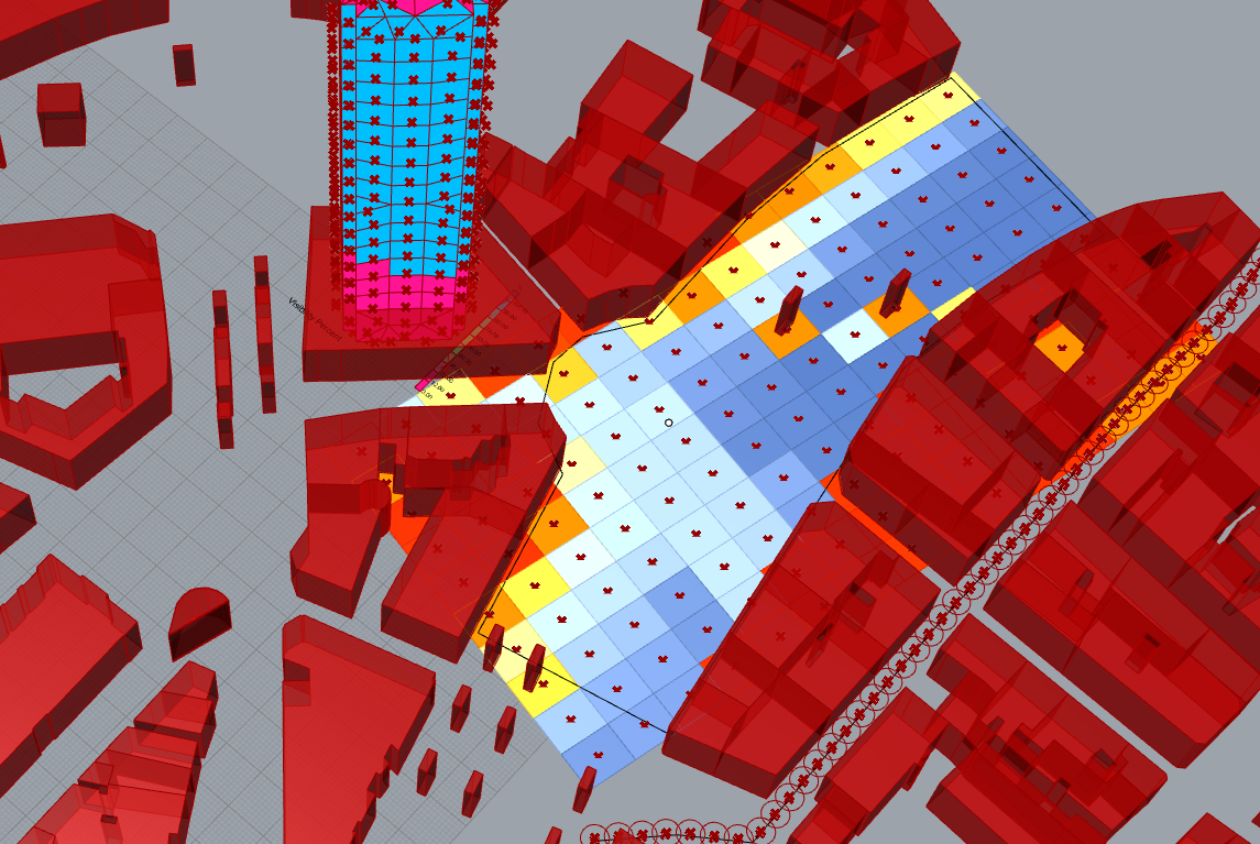
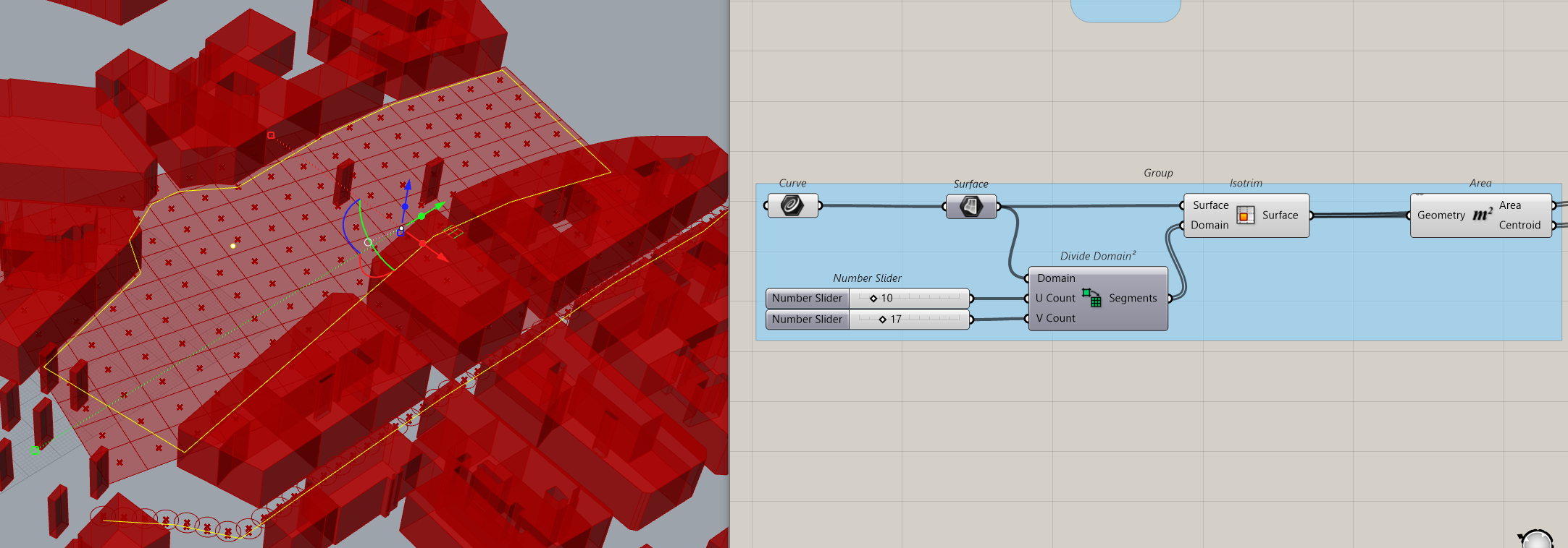
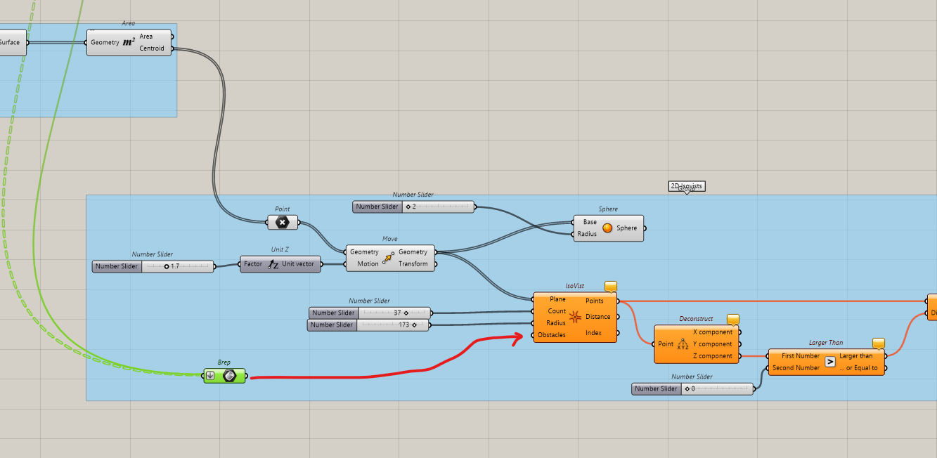
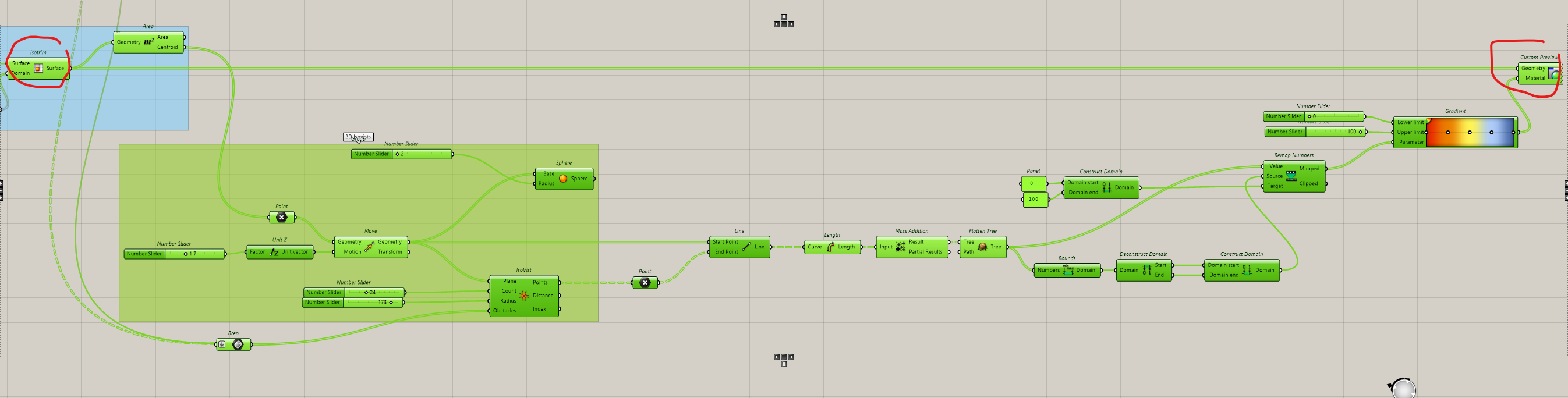
We can replace the path by a surface to investigate how much the tower is visible.

This is how is define our surface, it’s a simple setup for the test.

We connect the points to View_points and we add an offset to fit with the eye level

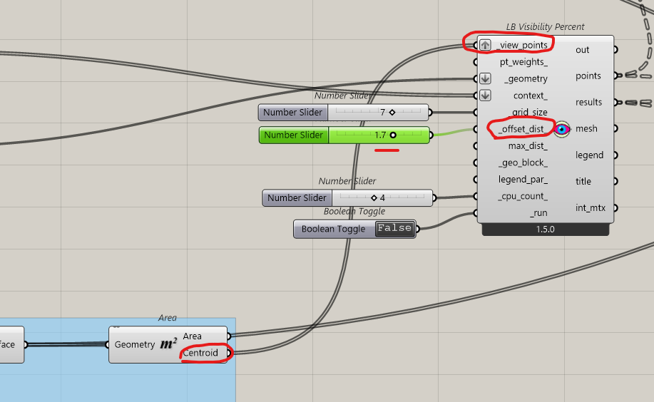
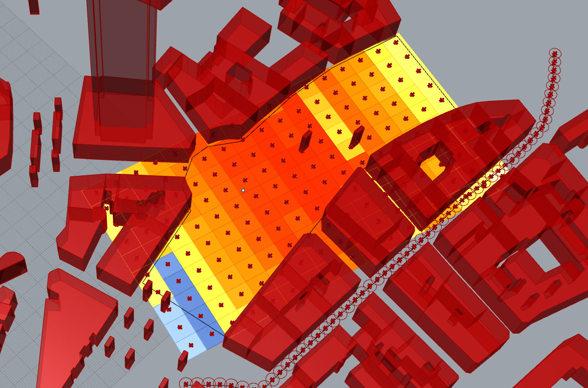
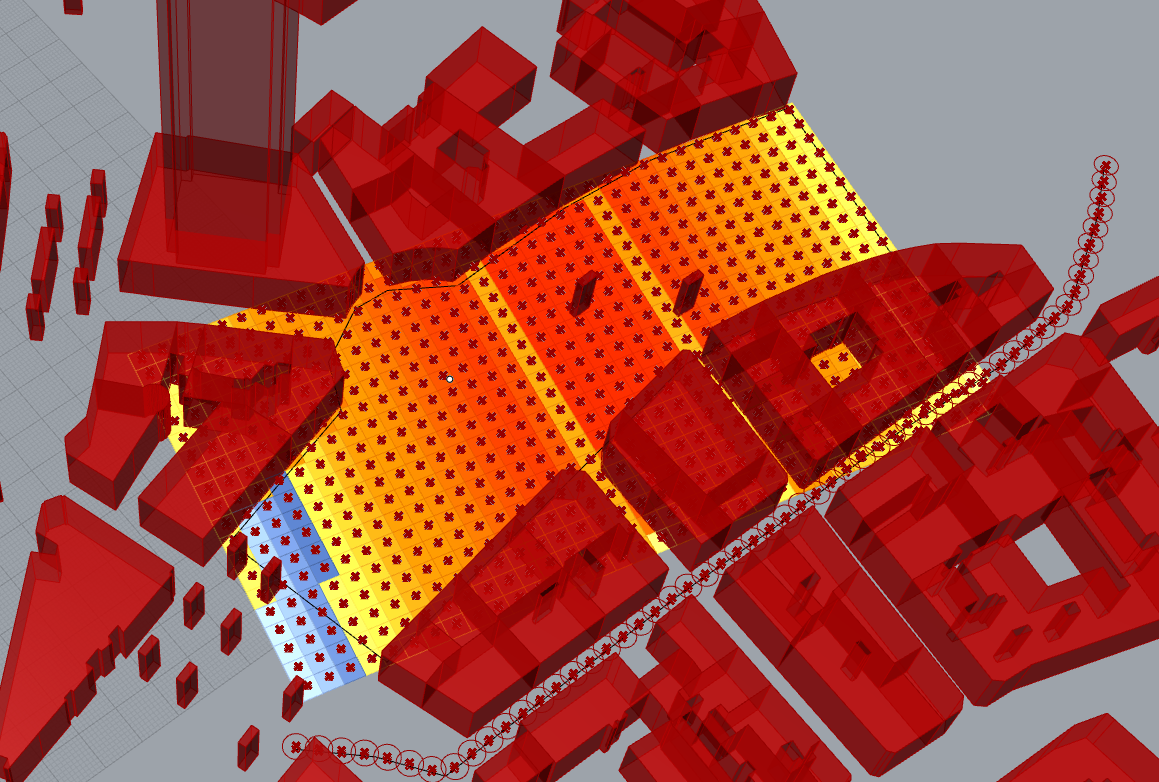
Result, the grid is large, (7 meters), we can try to get more details, but it will cost computer power

Last step, open visibilities.

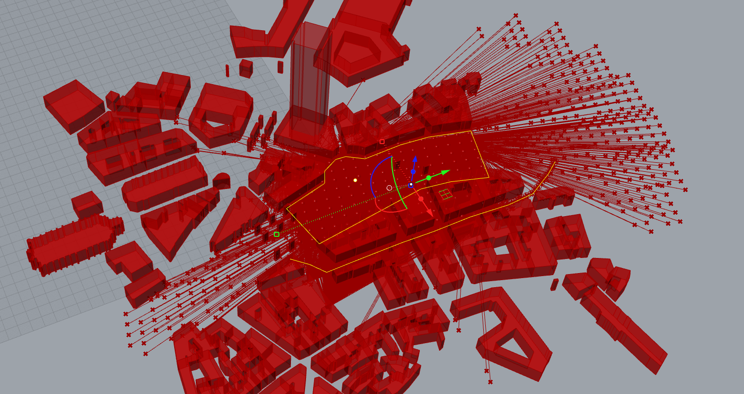
The perception of space can also derive from how far is it possible to see. Is density compatible with wider vision? We will see how to quantify this aspect using the first Isovist component we saw above.

We will create an Isovist for each point on this grid

We reuse the same definition

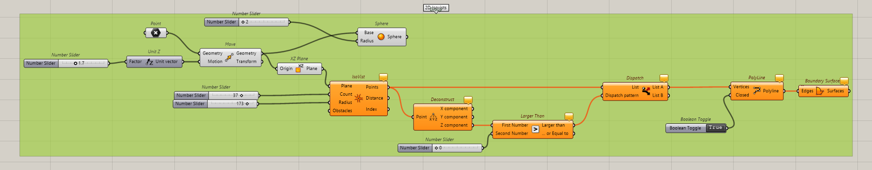
Connect every point of the grid to the Isovist definition

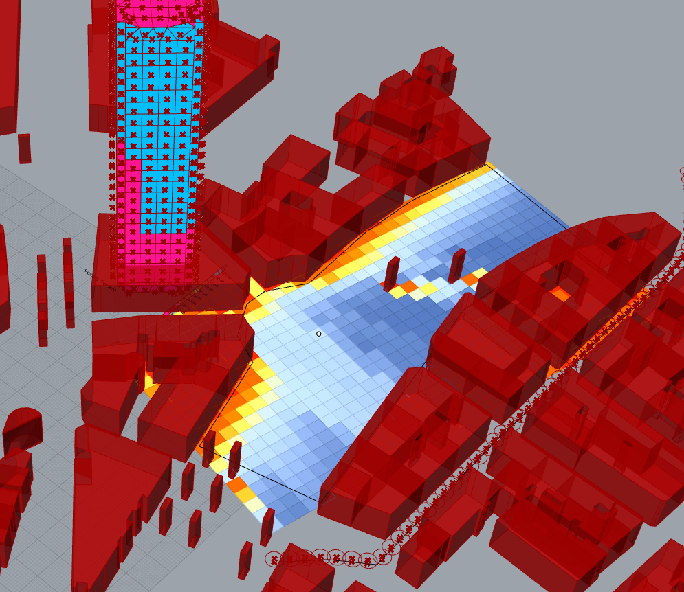
Now we could calculate the distance from each point to the first obstacle. The less it is, more confine is our space, and the more it is, more opened is our space.

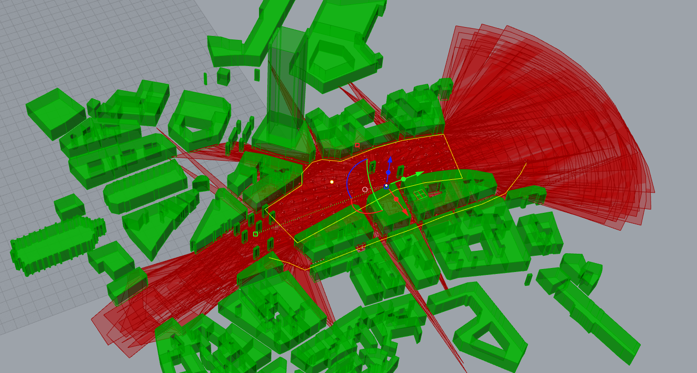
This is what we got.

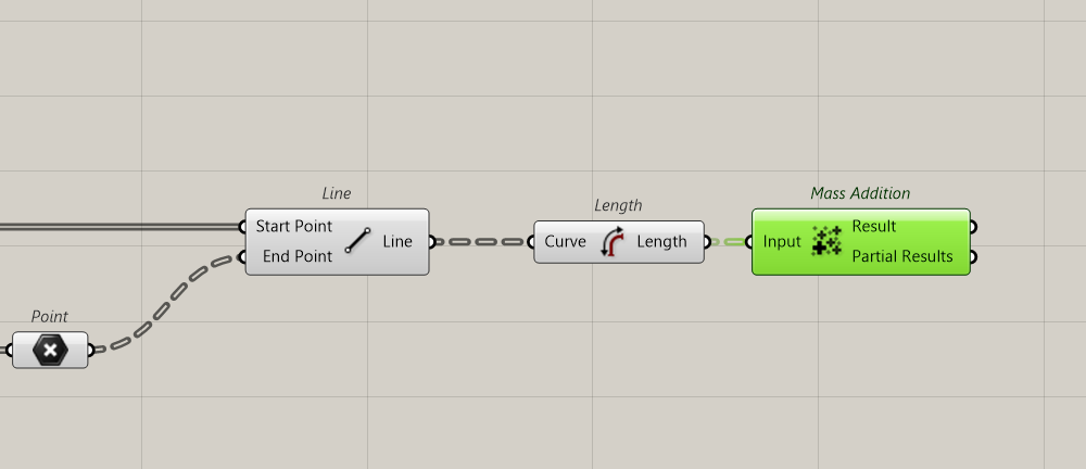
To make it more comprehensible, we will decrease the number of rays, and hide the surfaces and then create a segment for all rays.

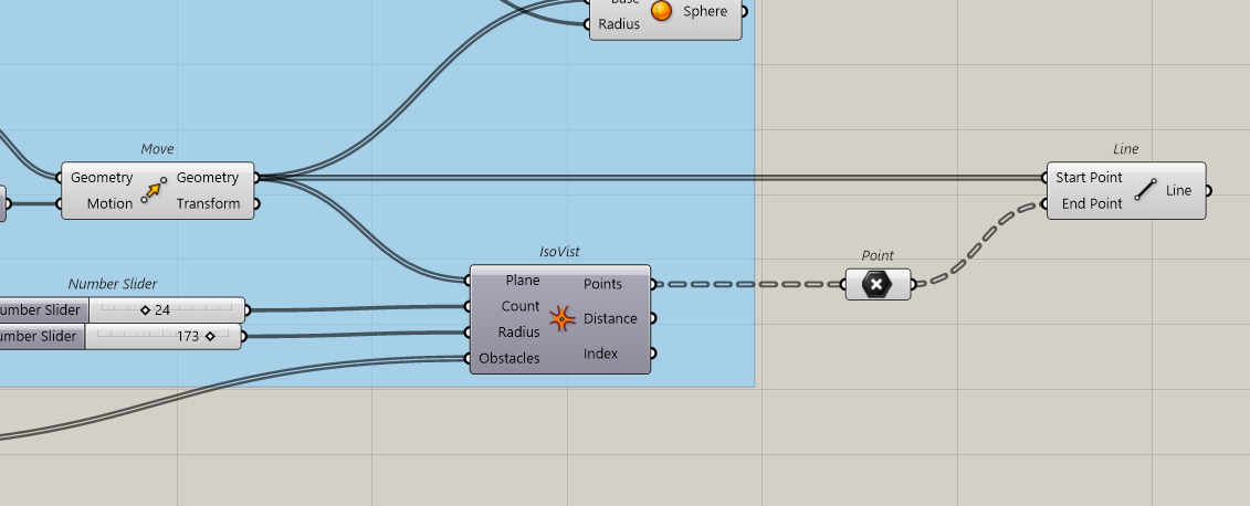
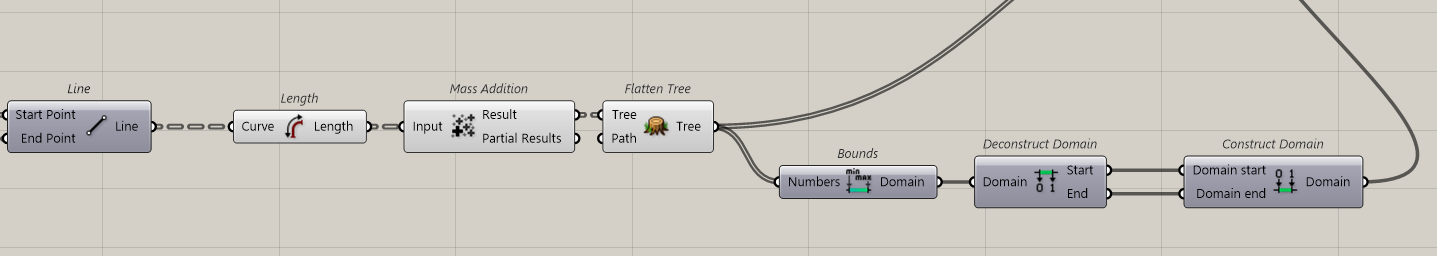
Now we will calculate every segment’s length and add them for each point.

We’ve here 170 points so 170 values

Ok, same as above we will create a colour from a gradient for each value.

We can reuse what has been done before.

So from the results, we look for the Min and Max value to create our Domain. We flatten the results and then look for the bounds and it gives our domain.

We remap our number for a more comfortable use, and input the Values.

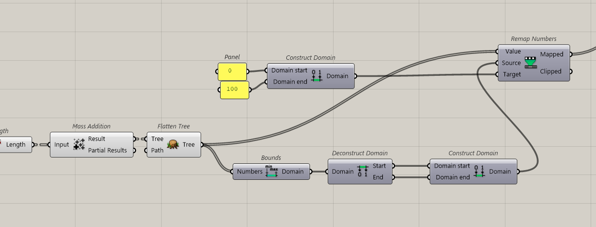
Then we connect to a gradient

Then those colours are distributed to all faces from our surface of study.

It’s done, this is our openness visibility study

Evaluate this lesson par filling the survey HERE