Photogrammetry helps the archeologist to have a accurate orthophotos where it can be very hard to install a camera. But instead of just getting the final result, it could also be interresting to record each step not only for visualisation but also for calculation.
![clip_image002[6]](http://www.keris-studio.fr/blog/wp-content/clip_image0026_thumb2.jpg "clip_image002[6]")
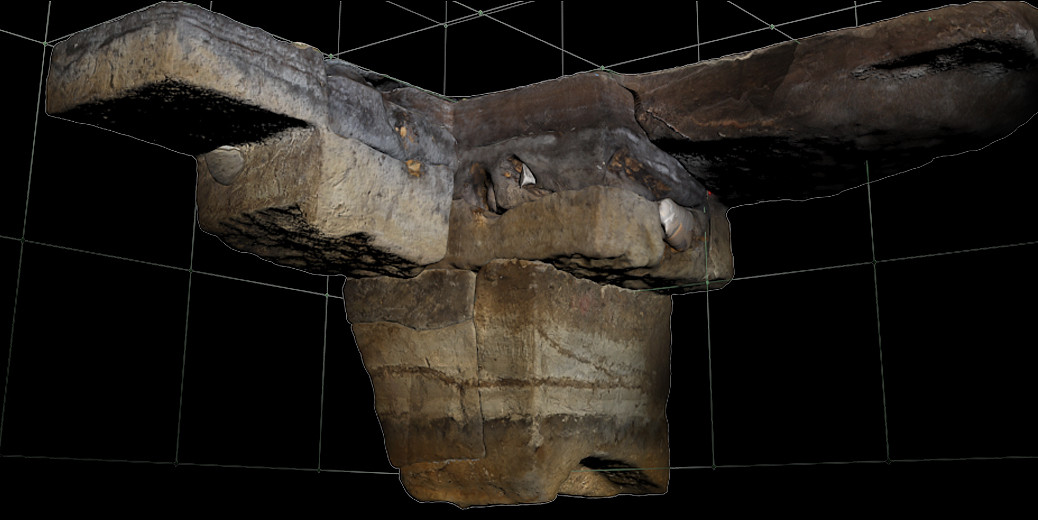
![clip_image002[4]](http://www.keris-studio.fr/blog/wp-content/clip_image002410.jpg "clip_image002[4]")
To say things fast, we wanted to record data between that :

… and that.

Before starting, the grid put on the ground has been used as a orthonormal. Three points were set : A(0,0,0), B(1,0,0) and C(0,1,0). Those points were then used in Photoscan to scale the model and stack all 3D geometry.

Simplification and export from Photoscan
The following work does not need a very dense geometry, it will be easier to process with a lighter model, but it’s necessary to keep a large texture for visual details.
In this example, I chose 10% as I knew I would have in the end a stack of 10 files with about 100 000 polygones each.


The texture has to be recalculate. When finished, the model can be exported in OBJ.
All layers, every step are gathered as shown below.

Step by step :


Superposition and visualisation of the excavation.
The following is done with Autodesk 3DsMax, but all kind of 3D software : Blender, Maya, Cinema 4D or Modo could be used the same way.
After importing, scale has to be checked.

All objects are grouped. When done, apply « Modifiers / Slice » and click on the (+) sign to make the « Slice Plane » Gizmo active. Rotate the Gizmo 90° and then clich on « Remove Top » or «Remove bottom » to see the slice..

Then apply « Edit Poly » ![]() and a « Shell ».
and a « Shell ».

Add an « Edit Poly » ![]() to modify the colour of slices. Select by angle.
to modify the colour of slices. Select by angle.

When selected, change « Material ID » set it to 2 for exemple. 
Set new materials as shown. Each slice gets a « Multi-sub Object » texture with in Slot 1, the original texture and in slot 2 the colour given the cut section .

Final result in perspective.

Final result as orthophoto.

Cut sections can also be colorized depending to the height.

Orthoview.

Quantities
Working with the void, it will be possible to determine some quantities.
Volumes.
This is easy to do using the last step.

The “hole” needs to be isolated

The top section is capped
The volume is calculated : 6,63 m3.
![]()
Calculation for each step.
All steps will be added starting from the very first one.

Step 0 will be the “lid” of the following step.

The “lid” is set over the geometry. Beware : faces underneath have to be flipped in order to fit with the top.

Step 1 and 2 are glued.


Next step :

The position of the root is clearly visible.

Next step :

Next one with a hard layer.

Last one.

All elements are grouped.


Summary Table
| Strata | Volume (m3) | Altitude
Sup (m) |
thikness
(cm) |
Nature |
 |
1,16 | 0,00 | 0,01->
0,50 max |
leaves & humus |
 |
0,16 | 0,00 | 0,01->
0,15 max |
leaves & humus |
 |
0,69 | -0,03
-0,20 |
0,04->
0,28 max |
Sand |
 |
0,88 | -0,28 | 0,40 | |
 |
0,69 | -0,10
-0,71 |
0,28
0,32 |
|
 |
0,35 | -0,96 | 0,19 | hard layer |
 |
0,86 | -0,01
-0,40 |
0,40
0,48 |
|
 |
0,98 | -1.17 | 0,68 | |
 |
1,63 | -0.03
-0.65 -0.96 -1.89 |
0,38max
0,31 1,09 0,24 |
Humus
sand |
 |
0,02 | -0,61 | Roots | |
| total | 7,49 |
Nota : the difference between above result and this one comes from the first layer of humus and leaves that has been taken in account before.
Geometry of each strata.
As example, this strata has been chosen :

Start by reversing faces then select.

One done, erase.

Then cap.

Volume is 0,1534m3 altitudes are -1,47m for the top face and -1,57m for the bottom one.
When finish it may look like this :


Bravo ! très impressionnant !
Mieux que ce que j’ai pu lire dans des articles payants de revues prestigieuses…
Merci de le mettre à disposition du plus grand nombre.
Une question : pourquoi de ne pas georéférencer le point de ref. ?
Oui en effet, il serait encore mieux de faire également le géoréférencement. De fait, chaque mission dégage de nouveaux besoins, de nouveaux processus et surtout de nouvelles précautions à prendre concernant la prise de vue, le recueil des données et l’organisation du travail. Vos commentaires sont précieux pour cela.